\(\theta\) control#
Hybrid model and switching law#
The following unified dynamics represents both the parallel and series resonant converters, where we recall that \(z=(z_1,z_2) \in \mathbb R^2\) is a physical state related to the current and voltage in the circuit, and \(\sigma \in \{-1,1\}\) is a logical state representing the position of the switch:
where \(A_F := \left[ \begin{smallmatrix} 0 & \omega\\ -\omega & -\beta\end{smallmatrix} \right]\), \(\omega>0\) is the natural frequency and \(\beta>0\) is the internal dissipation.
The sets \(\mathcal{C}\) and \(\mathcal{D}\) in (7) are called, respectively, flow set and jump set and are subsets of \(\mathbb R^2 \times \{-1,1\}\) whose intuitive meaning is that whenever the (augmented) state \(\xi:= (z, \sigma)\) belongs to \(\mathcal{D}\), it is time to change the switch position in the H-bridge driving the converter, whereas as long as \(\xi \in \mathcal{C}\), one may let the converter evolve continuously without changing the switch position. We design below \(\mathcal{C}\) and \(\mathcal{D}\), parametrized by a so-called switching angle \(\theta\in (0,\pi]\), representing a tuning knob of the proposed hybrid controller.
Following similar ideas to those in [Bonache-Samaniego et al., 2017], select the jump and the flow sets as
where each set \(\mathcal{C}_1\) and \(\mathcal{C}_{\mathrm{-}1}\) denotes a half plane and \(\mathcal{D}_1\) and \(\mathcal{D}_{\mathrm{-}1}\) are two half lines delimiting the flow sets, namely for each \(q\in \{1, \mathrm{-}1\}\),
The rationale behind the switching mechanism captured by (8) is illustrated in fig:illustration, where two possible trajectories are shown by projecting the three-dimensional state-space \((z_1,z_2,\sigma)\) on the phase plane \((z_1,z_2)\) (voltage, current). The left figure represents the case \(\theta< \frac{\pi}{2}\) while the right figure corresponds to \(\theta>\frac{\pi}{2}\).
During flowing (in \(\mathcal{C}(\theta)\)), the continuous evolution revolves in the clockwise direction. Switching always occurs when the continuous motion hits the tilted solid line.
When a switch occurs, the \(z_1\) voltage is shifted horizontally by two units, and the specific choice of \(\mathcal{C}(\theta)\) and \(\mathcal{D}(\theta)\) ensures that shifts always provide a clockwise rotation.
The choice to split \(\mathcal{D}\) in two half lines regularizes the domain avoiding Zeno solutions with \(\theta = \pi\). With this choice, after a solution jumps, it is forced to flow because it never lands again into the jump set.
The angle \(\theta\) controls the tilting of the blue-red line, namely the subspace where the switch takes place.
It is apparent that with small values of \(\theta\) (left case in fig:illustration) solutions
are forced to jump earlier when starting from the same initial condition.
Selection (8) provides a feedback control law. Indeed, checking whether or not the converter input should switch amounts to checking whether the state \(\xi=(z,\sigma)\) belongs to \(\mathcal{D}(\theta)\) or not. We show here that this feedback induces a self-oscillating behavior in the closed loop (7), (8).
Asymtotically Stable Hybrid Limit Cycle#
Main Stability Theorem#
According to [Bisoffi et al., 2018], the notion of periodicity for a hybrid trajectory is reported below. Alternative equivalent definitions are given in [Lou et al., 2018].
Definition 1
Given an hybrid system \(\mathcal{H}=(\mathcal{C},f,\mathcal{D},g)\), a nontrivial hybrid periodic trajectory \(\varphi\) is a complete solution (namely, a solution that evolves forever) that is not identically zero and for which there exists a pair \((T,J)\in \mathbb{R}_{\geq0} \times \mathbb{Z}_{\geq0}\) satisfying \(T+J>0\), such that \((t,j)\in\mathrm{dom}(\varphi)\) implies \((t+T,j+J)\in\mathrm{dom}(\varphi)\) and, moreover,
The image of \(\varphi\) is a nontrivial hybrid periodic orbit.
The next assumption on the parameters of (7) is necessary for the existence of a nontrivial hybrid periodic trajectory.
Assumption 1
Parameters \(\omega\) and \(\beta\) are strictly positive reals. Moreover, the relation \(\beta<2\omega\) is satisfied, namely the resonant tank is underdamped. Equivalently, the roots of \(s^2+\beta s+\omega^2=0\) are complex conjugate.
The following theorem, whose proof is reported in sec:proof, provides a justification for the proposed self-oscillating control law. In our preliminary work [Zaupa et al., 2021] we reported its proof only for the case \(\theta=\frac{\pi}{2}\). We prove it here for any value of \(\theta\in(0,\pi]\).
Theorem 1
Under Assumption 1, for each selection of \(\theta \in (0, \pi]\), the closed loop (7), (8) has a unique nontrivial hybrid periodic orbit \(\mathcal{O}_\theta\) that is stable and almost globally attractive (its basin of attraction includes all points such that \(z \neq 0\)). Moreover, the nontrivial hybrid periodic trajectories of (7), (8) are characterized by \(J=2\) and \(T(\theta)>0\), and exhibit periodic jumps interlaced by flowing intervals of length \(T(\theta)/2\).
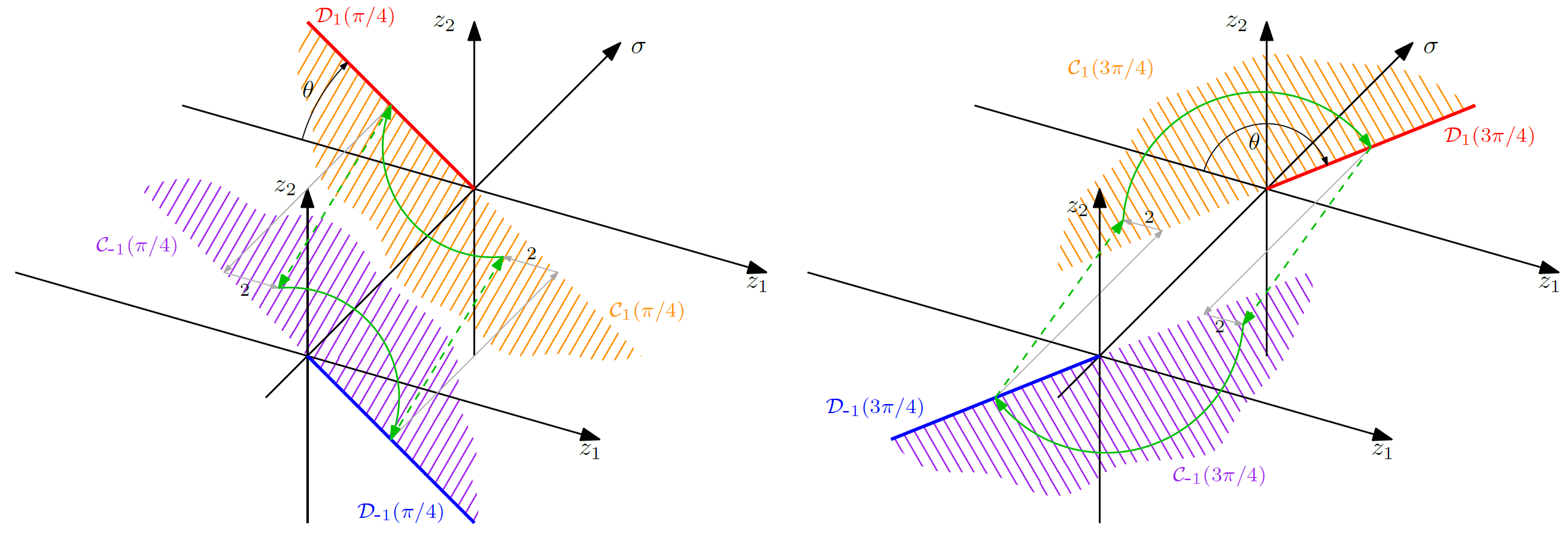
Fig. 2 Evolution of solutions and sets \({\mathcal G}_1\) (in green) and \(\mathcal{D}_1\) (in red) discussed in the proof of Theorem 1.#
Remark 1
Assumption 1 imposes constraints on the physical components to ensure that a natural oscillatory motion occurs, as certified by Theorem 1. For the two circuit configurations in Fig. 1, the constraint \(\beta<2\omega\) corresponds to:
Requirements (10) are reasonable since the effect of the load \(R\) must be sufficiently small to not destroy the natural oscillatory behavior of the \(LC\) resonant network. Ideally one would want, \(R\rightarrow\infty\) (open circuit) for the PRC and \(R\rightarrow0\) (short circuit) for the SRC. Both conditions in (10) can be stated in terms of quality factor \(Q\). Considering that \(Q_{\text{PRC}}=R\sqrt{\frac{C}{L}}\) and \(Q_{\text{SRC}}=\frac{1}{R}\sqrt{\frac{L}{C}}\) we have that:
which interestingly corresponds to the same requirement for both architectures. Constraint (11) immediately shows the advantage of our novel switching law, as compared to the alternative solutions of [Bonache-Samaniego et al., 2016, Bonache-Samaniego et al., 2017]. Indeed, a nontrivial discussion is present in [Bonache-Samaniego et al., 2016] showing for the PRC case that with \(Q < 3.15\) there is no guarantee of a self-oscillating behavior (the controller in [Bonache-Samaniego et al., 2016] may reach an equilibrium). The result of Theorem 1, only requiring the mild assumption (11) provides an important improvement.
Remark 2
The flow and jump sets of hybrid dynamics (7), (8) are closed, and the flow and jump maps are continuous functions, therefore (7), (8) enjoys the so-called hybrid basic conditions of As. 6.5 [Goebel et al., 2012]. This, among other things, implies robustness of asymptotic stability of compact attractors, as characterized in Ch. 7 [Goebel et al., 2012]. A consequence of robustness is that one expects a graceful degradation of the closed-loop stability properties (the so-called semiglobal practical robustness): an important feature for the experimental results discussed in Sections~\ref{sec:controller} and~\ref{sec:validation}.
Hybrid Lyapunov function and proof of Theorem 1#
In this section we prove Theorem 1, based on hybrid Lyapunov theory [Goebel et al., 2012]. Our proof shares interesting similarities with the approach reported in [Bisoffi et al., 2016] (see also [Bisoffi et al., 2018]), which address relay-based control of mechanical systems. In particular for the case \(\theta=\frac{\pi}{2}\) it is shown in [Zaupa et al., 2021] that Theorem 1 immediately follows from [Bisoffi et al., 2016]. Here we provide nontrivial derivations to allow extending the result to any \(\theta\in(0,\pi]\).
Before proving Theorem 1, let us recall from \cite[Def. 5.1]{convex} that a function \(\psi: \mathbb{R}\rightarrow\mathbb{R}\) is \(\alpha\)-strongly convex if and only if there exists \(\alpha>0\) such that for each \(a,b\in\mathbb{R}\) it holds that
where \(\partial\psi(b)\subset\mathbb{R}\) is the subdifferential of \(\psi\) at \(b\).
Based on (12) we can prove the following lemma, which is instrumental for the proof of Theorem 1.
Lemma 1
Consider two continuous functions of the scalar variable \(\xi\in\mathbb{R}_{\geq 0}\). A linear function \(\xi\mapsto \psi_1(\xi) = \psi_0 + \gamma\xi\), with \(\psi_0,\gamma\in\mathbb{R}\), and a strongly convex function \(\psi_2\) with \(\psi_2(0) < \psi_0\). Function \(\xi\mapsto\psi_1(\xi)-\psi_2(\xi)\) grows unbounded as \(\xi\rightarrow+\infty\) and has exactly one zero for \(\xi\geq 0\).
Proof. Denote \(\tilde\psi(\xi) := \psi_2 (\xi)-\psi_1 (\xi)\) and note that it is strongly convex because, for each \(a,b\in\mathbb{R}\) and each \(\sigma\in \partial \psi_2(b)\), it satisfies, from (12) applied with \(\psi=\psi_2\),
where \(\tilde\sigma=\sigma-\gamma\) characterizes any vector in the subdifferential of \(\tilde\psi\) at \(b\).
Let us first prove that function \(\tilde\psi\) has at least one zero for \(\xi\in[0,+\infty)\). From \(\psi_1(0) = \psi_0>\psi_2(0)\), we have \(\tilde\psi(0) < 0\). Applying (13) at the unique global minimum \(\xi^*\) (wherein \(\tilde\sigma=0\) belongs to \(\partial\tilde\psi (\xi^*))\), we have \(\tilde\psi (\xi) \geq\tilde\psi(\xi^*) +\frac{\alpha}{2} |\xi-\xi^*|^2\), which proves that \(\lim\limits_{\xi \to +\infty} \tilde\psi(\xi) = +\infty\), showing unboundedness of \(\psi(\xi)\) as \(\xi\rightarrow+\infty\). Moreover, with \(\tilde\psi(0) < 0\) and continuity, there exists at least one \(\xi_0\) where \(\tilde\psi(\xi_0) = 0\).
Let us now prove that \(\xi_0\) is unique. Assume that there are two points \(0 < \xi_0 < \xi_1\) where \(\tilde\psi\) is zero and fix \(a = \xi_1, b = \xi_0\). Then from (13) with these selections, we get:
which clearly implies \(\tilde\sigma<0\). Since \(\tilde\sigma\in\partial\tilde\psi(\xi_0)\) and \(\tilde\psi(\xi_0)=0\), by definition of subdifferential, using \(0<\xi_0\), we have \(\tilde\psi(0)\geq\tilde\psi(\xi_0)-\tilde\sigma\xi_0=-\tilde\sigma\xi_0>0\), which is a contradiction, because we proved above that \(\tilde\psi(0)<0\).
For proving Theorem 1, we formulate the following corollary of \cite[Lemma 1]{BisoffiECC16}, relating the dissipated energy along a flowing solution of (7), (8) to the hatched area in Fig. 2~(right).
Lemma 2
Consider any solution \(z\) to (7), (8) flowing from \(\mathcal{G}_{1}\) at ordinary time \(t_1\) to \(\mathcal{D}_1\) at ordinary time \(t_2>t_1\) and define energy-like function \(E(z)=\frac{1}{2}z_1^2 + \frac{1}{2}z_2^2 = \frac{1}{2}|z|^2\). The dissipated energy \(E(z(t_2))-E(z(t_1))\) is equal to \(\frac{\beta}{\omega}\Pi\), where \(\Pi\) is the (unsigned) area hatched between the graph of the trajectory \(z(t), \ t\in [t_1, t_2]\) and the coordinate axis \(z_2=0\).
Proof. Consider the following selection of the parameters and states in [Bisoffi et al., 2016]
From \cite[Lemma 1]{BisoffiECC16} the function \(E_{[21]}(x)=\frac{1}{2}\omega^2x_1^2 + \frac{1}{2}x_2^2 = \omega^2E(z)\) dissipates \(\Delta E_{[21]}=\beta\Pi_{[21]}\) between \(t_1\) and \(t_2\). From (15), in the \(z\) coordinates we have \(\Pi_{[21]}=\omega\Pi\) and since \(\Delta E_{[21]}=\omega^2\Delta E\), we have \(\Delta E = \frac{1}{\omega^2}\Delta E_{[21]} = \frac{\beta}{\omega^2}\Pi_{[21]} = \frac{\beta}{\omega}\Pi\) as to be proven.
To construct a Lyapunov function proving Theorem 1, let us only consider the half-space \(\mathcal{C}_1\), which also contains \(\mathcal{D}_1\) (parallel definitions apply to \(\mathcal{C}_{-1}\)) and introduce the set
which corresponds to the green-colored half line parallel to \(\mathcal{D}_{\mathrm{-}1}\) in Fig. 2. Then, for each point \(z \in\mathcal{C}_1\setminus\{0\}\), denote the compact time interval associated with the unique backward and forward flowing solutions of (7), flowing in \(\mathcal{C}_1\), as
where \([t_2,t_1]\) should be understood as the empty set when \(t_2>t_1\), so that \([\tau, 0] \cup [0,\tau]\) always describes an interval containing zero, whether \(\tau\) is positive or negative. Clearly, \(0 \in {\mathcal T}_1(z)\) for all \(z\in \mathcal{C}_1\setminus\{0\}\). Based on \({\mathcal T}_1(z)\), define the following two times, which exist and are unique for each \(z \in\mathcal{C}_1\setminus\{0\}\) due to the revolving nature of solutions, as per Assumption 1:
The Lyapunov function proposed in this proof, which is represented in Fig. 3 for the special case \(\theta = 3\pi/4\), is based on (17), (18) and corresponds to
where \(\Pi(z)\) has been defined in Lemma 2.
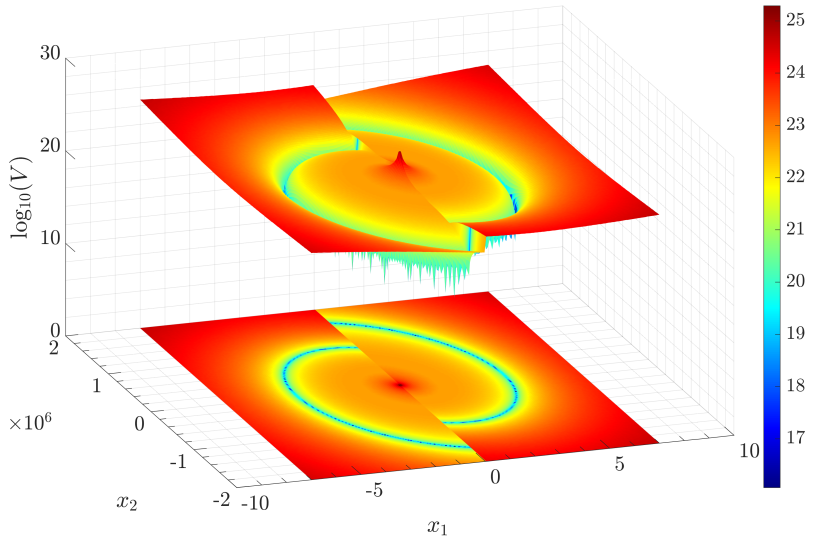
Fig. 3 Logarithmic representation of the Lyapunov function \(V\) in (19), for the value \(\theta = 3\pi/4\).#
The first term of \(V(z)\) in (19) is positive when \(z\) lies in the stripe between the set \(\mathcal{D}_{\mathrm{-}1}\) and \(\mathcal{G}_1\) of Fig. 2, wherein \(\tau_G(z)>0\), but it is zero in the remaining points of \(\mathcal{C}_1\), wherein \(\tau_G(z)\leq 0\). The second term of \(V(z)\) is inspired by [Bisoffi et al., 2016]. Referring to the energy \(E\) defined in Lemma 2, its numerator corresponds to the difference between the dissipated energy \(\frac{\beta}{\omega}\Pi(z)\) (sampled in a Poincar’e fashion) along the flow from \(\mathcal{G}_1\) to \(\mathcal{D}_1\) with the increase of energy across the jump from \(z_{1,D}= \left[ \begin{smallmatrix}1 & 0\end{smallmatrix} \right] {\mathrm e}^{A \tau_D(z)} z\), which belongs to \(\mathcal{D}_1\), namely
as defined in (20). Note that by construction \(\Pi\) and \(\delta_V\) are constant along flowing solutions, therefore, whenever {\(\tau_G(z)\leq0\)}, \(V\) remains constant along flowing solutions. Comparing \(\delta_V(z)\) with \(\frac{\beta}{\omega}\Pi(z)\), an energy balance between flows and jumps emerges when \(\delta_V(z)-\frac{\beta}{\omega}\Pi(z)=0\), that is when \(V(z)=0\). The denominator of the right term in (19) simply ensures that, close to the origin, \(V\) blows up to infinity, as it should because the origin is a weak equilibrium (it admits a constant flowing solution not converging to the hybrid periodic orbit) and cannot belong to the basin of attraction.
Defining \(V(z)\) in a parallel way for \(z\in\mathcal{C}_{\mathrm{-}1}\), we prove below that the following set, the zero level set of \(V\), corresponds to the set \(\mathcal{O}_\theta\) characterized in Theorem 1:
with \(\delta_V\) defined in (20). We are now ready to prove Theorem 1.
Proof. Let us first characterize function \(\Pi\), which is constant by construction along flowing solutions. Due to this fact we can parametrize all values of \(\Pi(z)\), \(z\in\mathcal{C}\cup\mathcal{D}\), following a Poincar’e approach for each \(z\in\mathcal{D}_1\), via \(\Pi(z)=\psi_2(|z|)\), where \(\psi_2(|z|)\) is the sum of the upper area \(\psi_2^{\mathrm{up}}(|z|)=\alpha^{\mathrm{up}}|z|^2\), which is homogeneous of degree two by construction, and the lower area \(\psi_2^{\mathrm{lw}} (|z|) = \alpha^{\mathrm{lw}}\max\left\lbrace|z|-|z_0| , 0\right\rbrace^2\), with \(z_0\in\mathcal{D}\) being the unique point such that \(\mathrm{e}^{A\tau_G(z_0)}z_0=\left[ \begin{smallmatrix} \mathrm{-}2\\0 \end{smallmatrix} \right]\), namely the point where \(\mathcal G_1\) has a kink, in Fig. 2. Due to homogeneity of the linear solutions (larger solutions are scaled versions of the smallest ones), it is immediate to see that \(\psi_2^{\mathrm{lw}}(|z|)\) is (non-strictly) convex and \(\psi_2^{\mathrm{up}}(|z|)\) is strongly convex. Therefore their sum is strongly convex. Let us continue by observing that for each \(z\in\mathcal{D}_1\), we can express the injected energy as
Then, from Lemma 1, there exists only one positive value {\(\xi^*=|z^*|\)} of \(|z|\) leading to the energy balance \(\psi_2(|z^*|)=\psi_1(|z^*|)\). In particular, the hybrid periodic orbit \(\mathcal{O}_\theta\) corresponds to the image of the hybrid periodic trajectory starting at the unique point \(z^*\in\mathcal{D}_1\).
By uniqueness of \(z^*\), the nontrivial hybrid periodic orbit \(\mathcal{O}_\theta\) is unique and coincides with set \(\mathcal{A}\) in (22).
Let us now prove the asymptotic stability of \(\mathcal A\) with basin of attraction \(\mathcal{B_A}= (\mathbb{R}^2\setminus\lbrace0\rbrace) \times \{-1,1\}\). To this end, let us first note that \(V\) is zero in \(\mathcal A\), positive in \(\mathcal{B_A}\) and, from Lemma 1, radially unbounded, relative to the open set \(\mathcal{B_A}\), with respect to \({\mathcal A}\). Moreover, since the points \({\mathrm e}^{A \tau_D(z)}z\) and \({\mathrm e}^{A \tau_G(z)}z\) remain constant along flowing solutions and \(\tau_G(z)\) is a decreasing function of time (due to the revolving nature of the solutions stemming from Assumption 1), then \(V\) in (19) is nonincreasing when flowing in \(\mathcal{C}\). Finally, from Lemma 1, and using similar arguments to those of \cite[Lemma 2]{BisoffiECC16}, the Lyapunov function decreases across jumps. More specifically, the following weak Lyapunov properties hold
As in [Bisoffi et al., 2016], the asymptotic stability of \({\mathcal A}\) with basin of attraction \(\mathcal{B_A}\) then follows from the nonsmooth hybrid invariance principle of Thm 1 from [Seuret et al., 2019].
The proof is completed by noting that, except for the trivial flowing solution at zero, the hybrid limit cycle whose orbit is \({\mathcal A}\), is globally attractive and therefore it is the only possible one. Moreover, due to the symmetry of the flow/jump sets and maps, this cycle is associated with periodic jumps, where the period \(T(\theta)\) of the jumps is given by the time it takes for a solution to reach \(\mathcal{D}_1\) from \({\mathcal G}_1\), along the periodic orbit. The period of the limit cycle is \((2T(\theta),2)\) because, by construction, it takes two half revolutions for the periodic trajectory starting in from \({\mathcal G}_1\) to revisit the same point in \({\mathcal G}_1\).