Unified model#
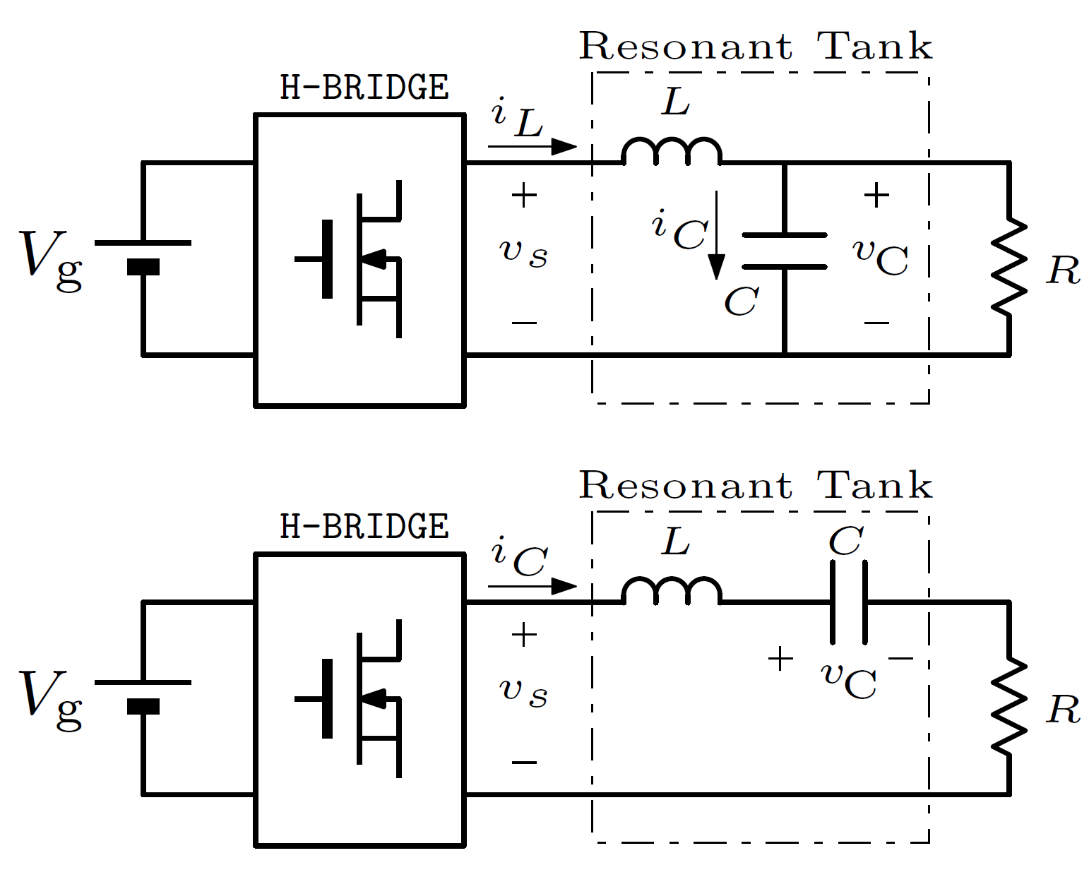
Fig. 1 Equivalent circuits associated with the parallel resonant converter (PRC, top) and series resonant converter (SRC, bottom).#
Unifying coordinate change#
We address parallel and series resonant converters (PRC and SRC, respectively), whose circuits are shown in Fig. 1, where \(v_C\) and \(i_C\) denote the voltage and the current in the capacitor. Both configurations exhibit a (parallel or series) resonant tank driven by an H-bridge applying a supply voltage \(v_s\) equal to either \(V_g\) or \(-V_g\) to the left terminal, where \(V_g\) is an external DC supply. The H-bridge is modeled here by a binary variable \(\sigma \in \{-1,1\}\) describing the switch position, so that \(v_s = V_g\) when \(\sigma =1\) and \(v_s = -V_g\) when \(\sigma = -1\) (in summary \(v_s = \sigma V_g\)).
The linear equations governing the current and voltage evolution of \(v_C\) and \(i_C\) for the parallel configuration at the top of Fig. 1 are the following ones:
We emphasize that the last term, \(\left( i_L -\frac{v_C}{R}\right)\), is the current \(i_C\) flowing in the capacitor. Similarly, the linear equations governing the series configuration at the bottom of Fig. 1 correspond to:
Note that in this case \(i_L=i_C\). The novel approach proposed there stems from introducing the next input-dependent quantities for the converters
the first one clearly corresponding to a transformed voltage and the second one being a transformed current.
Keeping in mind that any variation of \(\sigma \in \{-1, 1\}\) must be instantaneous, so that \(\dot \sigma = 0\), we may compute the differential equations governing the evolution of variables \(z:=(z_1,z_2)\) in (3). As shown in \cite{ADHS}, the dynamics is the same for the two circuits and corresponds to the following damped oscillator
where \(\omega := \left(\sqrt{LC}\right)^{-1}\) is the natural frequency and \(\beta>0\) is the inverse of the time constant of the exponential decay associated with each one of the linear circuits:
Since the coordinates \((z_1,z_2)\) depend on the input \(\sigma\), they experience an instantaneous change when \(\sigma\) is toggled. In particular, since \(\sigma\) toggles between \(-1\) and \(+1\), namely \(\sigma^+ = -\sigma\), then (3) provides, for both circuits:
where we emphasize that \(\sigma\) represents the switch position before the update and \(\sigma^+\) represents its position after the update (and similarly for the other variables).